Scan Conversion in Computer Graphics
Scan Conversion in Computer Graphics
“When we represent regular objects in the form of discrete pixels, it is called Scan Conversion.” Every graphics system must transform the primitives into a collection of pixels. The scan conversion is also called “Rasterization.” Each pixel in the graphical system has two states either on or off.
“The Scan Converting rate is a technique that is used in video processing. In this technique, we can change the horizontal and vertical frequency for many different purposes.” We use a scan converter to perform scan conversions. We can define a line by its starting and ending points. On the other hand, we can define a circle by its radius, circle equation, and center point.
Methods of Scan Conversion
We can perform scan conversion by using two methods.
- Analog Method
- Digital Method
- Analog Method: It is the best method for analog videos. A large number of delay cells perform the analog method. The Analog approach is also known as “Non-retentive, memory-less, or real-time method.”
- Digital Method: Digital method is also known as a “retentive or buffered method.” In the digital method, there is a concept of n1and n2 speed. We can save (Store) the picture in line or frame buffer with n1 speed. The image can be read with n2 speed.
Some Examples of scan converted objects
We can apply the conversion to the following objects.
- Line
- Point
- Polygon
- Rectangle
- Filled Region
- Arc
- Character
- Sector
- Ellipse
Advantages of Scan Conversion
- The scan conversion technique is used for various purposes, such as videoProjectors,TV, HDTV, Video capture card, LCD monitor, etc.
- The Scan Conversion technique has wide applications.
- We can efficiently perform scan conversion using high speed integrated circuits.
Disadvantages of Scan Conversion
- We can only apply scan conversion with LSI and VLSI integrated circuit.
- Int the digital scan conversion, the analog video signal has changed into digital data.
Line Drawing Algorithm in Computer Graphics
“The Line drawing algorithm is a graphical algorithm which is used to represent the line segment on discrete graphical media, i.e., printer and pixel-based media.”
A line contains two points. The point is an important element of a line.
Properties of a Line Drawing Algorithm
There are the following properties of a good Line Drawing Algorithm.
- An algorithm should be precise: Each step of the algorithm must be adequately defined.
- Finiteness: An algorithm must contain finiteness. It means the algorithm stops after the execution of all steps.
- Easy to understand: An algorithm must help learners to understand the solution in a more natural way.
- Correctness: An algorithm must be in the correct manner.
- Effectiveness: Thesteps of an algorithm must be valid and efficient.
- Uniqueness: All steps of an algorithm should be clearly and uniquely defined, and the result should be based on the given input.
- Input: A good algorithm must accept at least one or more input.
- Output: An algorithm must generate at least one output.
Equation of the straight line
We can define a straight line with the help of the following equation.
y= mx + a
Where,
(x, y) = axis of the line.
m = Slope of the line.
a = Interception point
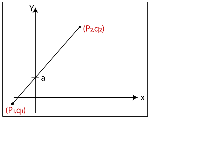
Let us assume we have two points of the line (p1, q1) and (p2, q2).
Now, we will put values of the two points in straight line equation, and we get
y = mx + a
q2 = mp2 ...(1)
q1 = mp1 + a ...(2)
We have from equation (1) and (2)
q2 – q1 = mp2 – mp1
q2 – q1 = m (p2 –p1)
The value of m = (q2 – q1)/ (p2 –p1)
m = ?q / ?p
Algorithms of Line Drawing
There are following algorithms used for drawing a line:
- DDA (Digital Differential Analyzer) Line Drawing Algorithm
- Bresenham’s Line Drawing Algorithm
DDA line Drawing Algorithm in Computer Graphics
DDA (Digital Differential Analyzer) Line Drawing Algorithm
The Digital Differential Analyzer helps us to interpolate the variables on an interval from one point to another point. We can use the digital Differential Analyzer algorithm to perform rasterization on polygons, lines, and triangles.
Digital Differential Analyzer algorithm is also known as an incremental method of scan conversion. In this algorithm, we can perform the calculation in a step by step manner. We use the previous step result in the next step.
As we know the general equation of the straight line is:
y = mx + c
Here, m is the slope of (x1, y1) and (x2, y2).
m = (y2 – y1)/ (x2 – x1)
Now, we consider one point (xk, yk) and (xk+1, yk+1) as the next point.
Then the slope m = (yk+1 - yk)/ (xk+1 - xk)
Now, we have to find the slope between the starting point and ending point. There can be following three cases to discuss:
Case 1: If m < 1
Then x coordinate tends to the Unit interval.
xk+1 = xk + 1
yk+1 = yk + m
Case 2: If m > 1
Then y coordinate tends to the Unit interval.
yk+1 = yk + 1
xk+1 = xk + 1/m
Case 3: If m = 1
Then x and y coordinate tend to the Unit interval.
xk+1 = xk + 1
yk+1 = yk + 1
We can calculate all intermediate points with the help of above three discussed cases.
Algorithm of Digital Differential Analyzer (DDA) Line Drawing
Step 1: Start.
Step 2: We consider Starting point as (x1, y1), and ending point (x2, y2).
Step 3: Now, we have to calculate ?x and ?y.
?x = x2-x1
?y = y2-y1
m = ?y/?x
Step 4: Now, we calculate three cases.
If m < 1
Then x change in Unit Interval
y moves with deviation
(xk+1, yk+1) = (xk+1, yk+1)
If m > 1
Then x moves with deviation
y change in Unit Interval
(xk+1, yk+1) = (xk+1/m, yk+1/m)
If m = 1
Then x moves in Unit Interval
y moves in Unit Interval
(xk+1, yk+1) = (xk+1, yk+1)
Step 5: We will repeat step 4 until we find the ending point of the line.
Step 6: Stop.
Example: A line has a starting point (1,7) and ending point (11,17). Apply the Digital Differential Analyzer algorithm to plot a line.
Solution: We have two coordinates,
Starting Point = (x1, y1) = (1,7)
Ending Point = (x2, y2) = (11,17)
Step 1: First, we calculate ?x, ?y and m.
?x = x2 – x1 = 11-1 = 10
?y = y2 – y1 = 17-7 = 10
m = ?y/?x = 10/10 = 1
Step 2: Now, we calculate the number of steps.
?x = ?y = 10
Then, the number of steps = 10
Step 3: Weget m = 1, Third case is satisfied.
Now move to next step.
| xk | yk | xk+1 | yk+1 | (xk+1, yk+1) |
| 1 | 7 | 2 | 8 | (2, 8) |
| 3 | 9 | (3, 9) | ||
| 4 | 10 | (4, 10) | ||
| 5 | 11 | (5, 11) | ||
| 6 | 12 | (6, 12) | ||
| 7 | 13 | (7, 13) | ||
| 8 | 14 | (8, 14) | ||
| 9 | 15 | (9, 15) | ||
| 10 | 16 | (10, 16) | ||
| 11 | 17 | (11, 17) |
Step 4: We will repeat step 3 until we get the endpoints of the line.
Step 5: Stop.
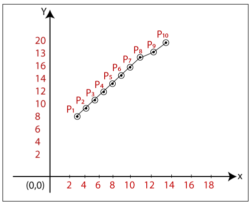
The coordinates of drawn line are-
P1 = (2, 8)
P2 = (3, 9)
P3 = (4, 10)
P4 = (5, 11)
P5 = (6, 12)
P6 = (7, 13)
P7 = (8, 14)
P8 = (9, 15)
P9 = (10, 16)
P10 = (11, 17)
Advantages of Digital Differential Analyzer
- It is a simple algorithm to implement.
- It is a faster algorithm than the direct line equation.
- We cannot use the multiplication method in Digital Differential Analyzer.
- Digital Differential Analyzer algorithm tells us about the overflow of the point when the point changes its location.
Disadvantages of Digital Differential Analyzer
- The floating-point arithmetic implementation of the Digital Differential Analyzer is time-consuming.
- The method of round-off is also time-consuming.
- Sometimes the point position is not accurate.
Bresenham’s Line Drawing Algorithm in Computer Graphics
This algorithm was introduced by “Jack Elton Bresenham” in 1962. This algorithm helps us to perform scan conversion of a line. It is a powerful, useful, and accurate method. We use incremental integer calculations to draw a line. The integer calculations include addition, subtraction, and multiplication.
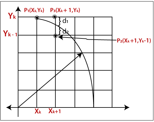
In Bresenham’s Line Drawing algorithm, we have to calculate the slope (m) between the starting point and the ending point.
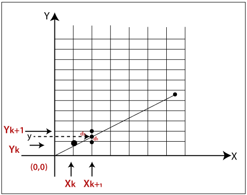
As shown in the above figure let, we have initial coordinates of a line = (xk, yk)
The next coordinates of a line = (xk+1, yk+1)
The intersection point between yk and yk+1 = y
Let we assume that the distance between y and yk = d1
The distance between y and yk+1 = d2
Now, we have to decide which point is nearest to the intersection point.
If m < 1
then x = xk+1 { Unit Interval}
y = yk+1 { Unit Interval}
As we know the equation of a line-
y = mx +b
Now we put the value of x into the line equation, then
y = m(xk+1) +b …………. (1)
The value of d1 = y - yk
Now we put the value of d1 in equation (1).
y = m (xk+1) +b - yk
Now, we again put the value of y in the previous equation then we got,
d2 = yk+1 – y
= yk + 1 – m (xk+1) – b
Now, we calculate the difference between d1 – d2
If d1 < d2
Then yk+1 = yk {we will choose the lower pixel as shown in figure}
If d1 => d2
Then yk+1 = yk+1 {we will choose the upper pixel as shown in figure}
Now, we calculate the values of d1 - d2
(d1 - d2)= m (xk+1) +b - yk - yk - 1 + m (xk+1) + b
We simplified the above equation and replaced the m with ?y/?x.
(d1 - d2) = 2 m (xk+1) -2yk + 2b-1
We multiplied ?x at both side then we got,
?x (d1 - d2) = ?x (2m (xk+1) -2yk + 2b-1)
We consider ?x (d1 - d2) as a decision parameter (Pk), so
pk = ?x (d1 - d2)
After calculation we got,
Pk = 2?yxk + 2?y - 2?xyk +?x (2b-1)
Then, the next coordinate of pk
pk+1 = 2?yxk+1 + 2?y - 2?xyk+1 +?x (2b-1)
Now, the difference between pk+1 – pk then,
pk+1 – pk = 2?y (xk+1-xk) – 2?x (yk+1-yk)
pk+1 = pk + 2?y (xk+1-xk) – 2?x (yk+1-yk) {Decision parameter coordinate}
Now, we put the value of xk+1 in above equation then we got,
pk+1 = pk + 2?y – 2?x (yk+1 - yk) {New decision parameter when m <1}
Similarly, if m >1, the new decision parameter for next coordinate will be
pk+1 = pk + 2?y – 2?x (xk+1 - xk) {New decision parameter when m >1}
If pk >= 0 {For coordinate y}
Then,
yk+1 = yk+1 {We will choose the nearest yk+1 pixel}
The next coordinate will be (xk+1, yk+1)
If pk < 0
Then,
yk+1 = yk {We will choose the nearest yk pixel}
The next coordinate will be (xk+1, yk)
Similarly,
If pk >= 0 {For coordinate x}
Then,
xk+1 = xk+1 {We will choose the nearest xk+1 pixel}
The next coordinate will be (xk+1, yk+1)
If pk < 0
Then,
xk+1 = xk {We will choose the nearest xk pixel}
The next coordinate will be (xk, yk+1)
Algorithm of Bresenham’s Line Drawing Algorithm
Step 1: Start.
Step 2: Now, we consider Starting point as (x1, y1) and endingpoint (x2, y2).
Step 3: Now, we have to calculate ?x and ?y.
?x = x2-x1
?y = y2-y1
m = ?y/?x
Step 4: Now, we will calculate the decision parameter pk with following formula.
pk = 2?y-?x
Step 5: Theinitial coordinates of the line are (xk, yk), and the next coordinatesare (xk+1, yk+1). Now, we are going to calculate two cases for decision parameter pk
Case 1: If
pk < 0
Then
pk+1 =pk +2?y
xk+1 = xk +1
yk+1 = yk
Case 2: If
pk >= 0
Then
pk+1 =pk +2?y-2?x
xk+1 =xk +1
yk+1 =yk +1
Step 6: We will repeat step 5 until we found the ending point of the line and the total number of iterations =?x-1.
Step 7: Stop.
Example: A line has a starting point (9,18) and ending point (14,22). Apply the Bresenham’s Line Drawing algorithm to plot a line.
Solution: We have two coordinates,
Starting Point = (x1, y1) = (9,18)
Ending Point = (x2, y2) = (14,22)
Step 1: First, we calculate ?x, ?y.
?x = x2 – x1 = 14-9 = 5
?y = y2 – y1 = 22-18 = 4
Step 2: Now, we are going to calculate the decision parameter (pk)
pk = 2?y-?x
= 2 x 4 – 5 = 3
The value of pk = 3
Step 3: Now, we will check both the cases.
If
pk >= 0
Then
Case 2 is satisfied. Thus
pk+1 = pk +2?y-2?x =3+ (2 x 4) - (2 x 5) = 1
xk+1 =xk +1 = 9 + 1 = 10
yk+1 =yk +1 = 18 +1 = 19
Step 4: Now move to next step. We will calculate the coordinates until we reach the end point of the line.
?x -1 = 5 – 1 = 4
pk pk+1 xk+1 yk+1 9 18 3 1 10 19 1 -1 11 20 -1 7 12 20 7 5 13 21 5 3 14 22 Step 5: Stop.

The Coordinates of drawn lines are-
P1 = (9, 18)
P2 = (10, 19)
P3 = (11, 20)
P4 = (12, 20)
P5 = (13, 21)
P6 = (14, 22)
Advantages of Bresenham’s Line Drawing Algorithm
- It is simple to implement because it only contains integers.
- It is quick and incremental
- It is fast to apply but not faster than the Digital Differential Analyzer (DDA) algorithm.
- The pointing accuracy is higher than the DDA algorithm.
Disadvantages of Bresenham’s Line Drawing Algorithm
- The Bresenham’s Line drawing algorithm only helps to draw the basic line.
- The resulted draw line is not smooth.
Scan Conversion of a Circle Computer Graphics
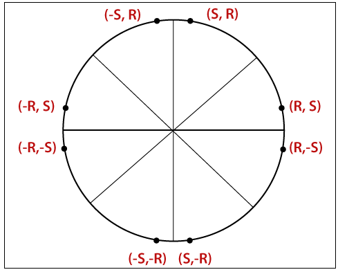
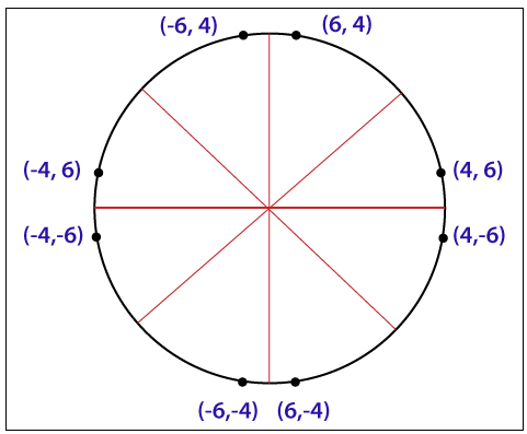
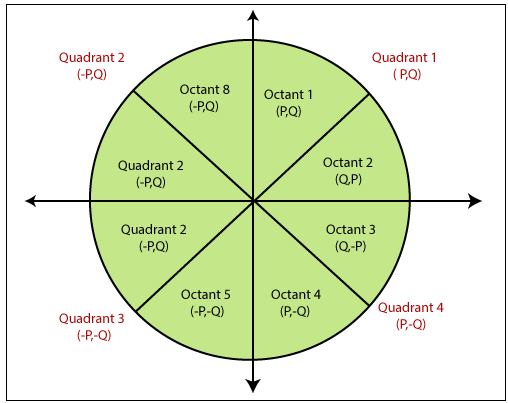
A circle is an eight-way symmetric shape. All quadrants of a circle are the same. There are two octants in each quadrant of a circle. If we know the value of any point, then we can easily calculate the values of the remaining seven points by using the eight-way symmetry method. A circle is a shape consist of a line called the circumference. All the straight lines drawn from a particular point within the circle to the circumference are always equal. A circle is a round shape that has no corner or sides.
“A circle can be defined as a combination of points that all points are at the same distance (radius) from the center point.” We can express a circle by the following equation-
(P - Pc)2 + (Q - Qc)2 = r2
The above equation can be written as-
(P)2 + (Q)2 = r2 {r = radius}
If we want to draw a circle, then we will consider it by its origin point. Let us assume a point P1(R, S) then we can represent the other seven points as follows-
P2(R, -S)
P3(-R, -S)
P4(-R, S)
P5(S, R)
P6(S, -R)
P7(-S, -R)
P8(-S, R)
We can also represent eight points of the circle on the computer screen by using of put pixel function ().
Putpixel (R, S, Color)
Putpixel (R, -S, Color)
Putpixel (-R, -S, Color)
Putpixel (-R, S, Color)
Putpixel (R, S, Color)
Putpixel (R, -S, Color)
Putpixel (-R, -S, Color)
Putpixel (-R, S, Color)
Example: Let, we have taken a point (4, 6) of a circle. We will calculate the remaining seven points by using of reflection method as follows-
The seven points are – (4, -6), (-4, -6), (-4, 6), (4, 6), (4, -6), (-4, -6), (-4, 6)
There are two following standard methods to define a circle mathematically.
- A circle with a second-order polynomial equation.
- A circle with trigonometric/ polar coordinates.
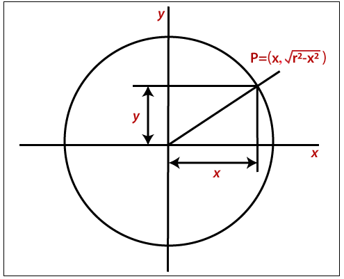
A circle with the second-order polynomial equation-
y2 =r2 – x2
Here, x = The coordinates of x
y = The coordinates of y
r = The radius of the circle
In this method, we will find the x coordinate (90° to 45°) by moving x from 0 to r/?2, and we will find each y coordinate by calculating ?r2-x2 for each step.
It is an ineffective method because for each point x coordinate and radius r must be squaredand subtracted from each other.
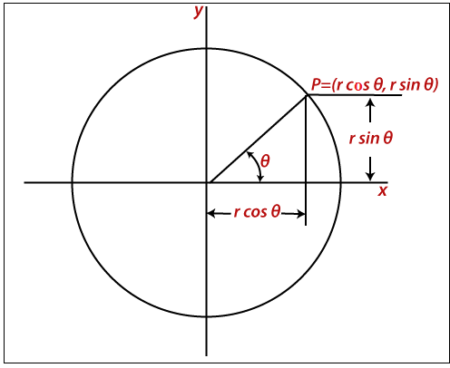
A circle with trigonometric/polar coordinate-
x = r cos ?
y = r sin ?
Here, x = The coordinate of x
y = The coordinate of y
r = The radius of the circle
? = Current angle
In this method, the value of ? moves from 0 to ?/4. We will calculate each value of x and y.
Algorithms used in Circle Drawing
There are the following two algorithms used to draw a circle.
- Bresenham’s Circle drawing Algorithm
- Mid-point Circle Drawing Algorithm
Bresenham’s Circle Drawing Algorithm in Computer Graphics
Bresenham’s algorithm is also used for circle drawing. It is known as Bresenham’s circle drawing algorithm. It helps us to draw a circle. The circle generation is more complicated than drawing a line. In this algorithm, we will select the closest pixel position to complete the arc. We cannot represent the continuous arc in the raster display system. The different part of this algorithm is that we only use arithmetic integer. We can perform the calculation faster than other algorithms.
Let us assume we have a point p (x, y) on the boundary of the circle and with r radius satisfying the equation fc (x, y) = 0
As we know the equation of the circle is –
fc (x, y) = x2 + y2 = r2
If
fc (x, y) < 0
then
The point is inside the circle boundary.
If
fc (x, y) = 0
then
The point is on the circle boundary.
If
fc (x, y) > 0
then
The point is outside the circle boundary.
We assume,
The distance between point P3 and circle boundary = d1
The distance between point P2 and circle boundary = d2
Now, if we select point P3 then circle equation will be-
d1 = (xk +1)2 + (yk)2 – r2 {Value is +ve, because the point is outside the circle}
if we select point P2 then circle equation will be-
d2 = (xk +1)2 + (yk -1)2 – r2 {Value is -ve, because the point is inside the circle}
Now, we will calculate the decision parameter (dk) = d1 + d2
dk =(xk +1)2 + (yk)2 – r2 + d2 + (xk +1)2 + (yk -1)2 – r2
= 2(xk +1)2 + (yk)2+ (yk -1)2 – 2r2 …………………… (1)
If
dk < 0
then
Point P3 is closer to circle boundary, and the final coordinates are-
(xk +1, yk) = (xk +1, yk)
If
dk >= 0
then
Point P2 is closer to circle boundary, and the final coordinates are-
(xk +1, yk) = (xk +1, yk -1)
Now, we will find the next decision parameter (dk+1)
(dk+1) = 2(xk+1 +1)2 + (yk+1)2+ (yk+1 -1)2 – 2r2 …………………… (2)
Now, we find the difference between decision parameter equation (2) - equation (1) (dk+1) – (dk) = 2(xk+1+1)2 + (yk+1)2+ (yk+1 –1)2 – 2r2 – 2(xk +1)2 + (yk)2+ (yk– 1)2 – 2r2 (dk+1) = dk + 4xk + 2(yk+12– yk2) – (yk+1 – yk) + 6
Now, we check two conditions for decision parameter-
Condition 1: If
dk < 0
then
yk+1 = yk (We select point P3)

Condition 2: If
dk >= 0
then
yk+1 = yk-1 (We select point P3)
Now, we calculate initial decision parameter (d0)

d0 = d1 + d2
d0 = {12 +r2– r2} + {12 +(r – 1)2 – r2}
d0 = 3 – 2r

Algorithm of Bresenham’s Circle Drawing
Step 1: Start.
Step 2: First, we allot the starting coordinates (x1, y1) as follows-
x1 = 0
y1 =r
Step 3: Now, we calculate the initial decision parameter d0 -
d0 = 3 – 2 x r
Step 4: Assume,the initial coordinates are (xk, yk)
The next coordinates will be (xk+1, yk+1)
Now, we will find the next point of the first octant according to the value of the decision parameter (dk).
Step 5: Now, we follow two cases-
Case 1: If
dk < 0
then
xk+1 =xk + 1
yk+1 =yk
dk+1 = dk + 4xk+1 + 6
Case 2: If
dk >= 0
then
xk+1 =xk + 1
yk+1 =yk –1
dk+1 = dk + 4(xk+1 – yk+1)+ 10
Step 6: If the center coordinates (x1, y1) is not at the origin (0, 0), then we will draw the points as follow-
X coordinate = xc + x1
y coordinate = yc + y1 {xc andyc representsthe current value of x and y coordinate}
Step 7: We repeat step 5 and 6 until we get x>=y.
Step 8: Stop.
Example: The radius of a circle is 8, and center point coordinates are (0, 0). Apply bresenham’s circle drawing algorithm to plot all points of the circle.
Solution:
Step 1: The given stating points of the circle (x1, y1) = (0, 0)
Radius of the circle (r) = 8
Step 2: Now, we will assign the starting point (x1, y1) as follows-
x1 = 0
y1 = r (radius) = 8
Step 3: Now, we will calculate the initial decision parameter (d0)
d0 = 3 – 2 x r
d0 = 3 – 2 x 8
d0 = -13
Step 4: The value of initial parameter d0 < 0. So, case 1 is satisfied.
Thus,
xk+1 =xk + 1 = 0 + 1 = 1
yk+1 =yk = 8
dk+1 = dk + 4xk+1 + 6 = -13 + (4 x 1) + 6 = -3
Step 5: The center coordinates are already (0, 0) so we will move to next step.
Step 6: Follow step 4 until we get x >= y.
Table for all points of octant 1:
dk dk+1 (xk+1,yk+1) (0, 8) -13 -3 (1, 8) -3 11 (2, 8) 11 5 (3, 7) 5 7 (4, 6) 7 (5, 5) Now, we will calculate the coordinates of the octant 2 by swapping the x and y coordinates.
Coordinates of Octant 1 Coordinates of Octant 2 (0, 8) (5, 5) (1, 8) (6, 4) (2, 8) (7, 3) (3, 7) (8, 2) (4, 6) (8, 1) (5, 5) (8, 0) Thus, we will calculate all points of the circle with respect to octant 1.
Quadrant 1 (x, y) Quadrant 2 (-x, y) Quadrant 3 (-x, -y) Quadrant 4 (x, -y) (0, 8) (0, 8) (0, -8) (0, -8) (1, 8) (-1, 8) (-1, -8) (1, -8) (2, 8) (-2, 8) (-2, -8) (2, -8) (3, 7) (-3, 7) (-3, -7) (3, -7) (4, 6) (-4, 6) (-4, -6) (4, -6) (5, 5) (-5, 5) (-5, -5) (5, -5) (6, 4) (-6, 4) (-6, -4) (6, -4) (7, 3) (-7, 3) (-7, -3) (7, -3) (8, 2) (-8, 2) (-8, -2) (8, -2) (8, 1) (-8, 1) (-8, -1) (8, -1) (8, 0) (-8, 0) (-8, 0) (8, 0) Advantages of Bresenham’s Circle Drawing Algorithm
- It is simple and easy to implement.
- The algorithm is based on simple equation x2 + y2 = r2.
Disadvantages of Bresenham’s Circle Drawing Algorithm
- The plotted points are less accurate than the midpoint circle drawing.
- It is not so good for complex images and high graphics images.
Midpoint Circle Drawing Algorithm in Computer Graphics
The midpoint circle drawing algorithm helps us to calculate the complete perimeter points of a circle for the first octant. We can quickly find and calculate the points of other octants with the help of the first octant points. The remaining points are the mirror reflection of the first octant points.
This algorithm is used in computer graphics to define the coordinates needed for rasterizing the circle. The midpoint circle drawing algorithm helps us to perform the generalization of conic sections. Bresenham’s circle drawing algorithm is also extracted from the midpoint circle drawing algorithm. In the algorithm, we will use the 8-way symmetry property.
In this algorithm, we define the unit interval and consider the nearest point of the circle boundary in each step.
Let us assume we have a point a (p, q) on the boundary of the circle and with r radius satisfying the equation fc (p, q) = 0
As we know the equation of the circle is –
fc (p, q) = p2 + q2 = r2 …………………………… (1)
If
fc (p, q) < 0
then
The point is inside the circle boundary.
If
fc (p, q) = 0
then
The point is on the circle boundary.
If
fc (p, q) > 0
then
The point is outside the circle boundary.
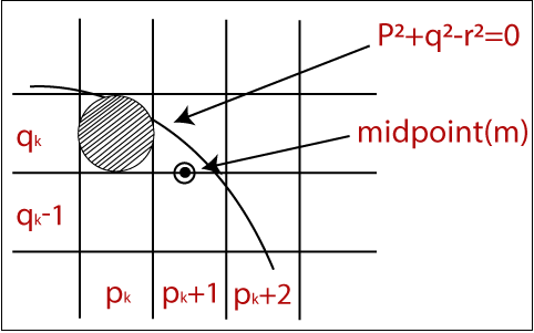
In the figure, we calculate the mid-point (m). The midpoint appears between qk and qk -1.
The currentposition of the pixel = pk +1
The next position of the pixel = (pk +1, qk) and (pk +1, qk - 1)
Now, we will calculate the decision parameter (dk)
dk = (pk +1, qk – 1/2)
Now, we replace all the values with equation (1)
dk = (pk +1)2 + (qk – 1/2)2 – r2 …………………………………… (2)
Now, there should be two conditions.
Condition 1: If
dk is negative
then
The midpoint (m) is inside the circle boundary
Condition 2: If
dk is positive
then
The midpoint (m) is outside the circle boundary
Now, we find the next point of x coordinates. Then,
Pk+1 +1 = Pk+2
Now, we replace all the value of equation (2) with (k+1). We get-
dk+1 = (pk+1 +1)2 + (qk+1 – 1/2)2 – r2 ……………………………. (3)
Now, we will find the difference between
dk+1 – dk = {(pk+1 +1)2 + (qk+1 – 1/2)2 – r2} – {(pk +1)2 + (qk – 1/2)2 – r2}
= dk +(2pk +1) + (qk+12 – qk2) – (qk+1 – qk) +1 …………………… (4)
Here, If
dk isnegativethen dk+1
then
2pk+1 +1
Otherwise
2pk+1 +1 – 2qk+1
Now, the next coordinate for x and y points
2pk+1 = 2pk +2
2qk+1 = 2qk –2
Now, the initial decision parameter (d0) at the position (p, q) = (0, r)
We put (0, r) in circle equation and we get-
d0 = (1, r – 1/2)
= (1 + (r –1/2)2 –r2)
= 5/4 –r
We only take integer value = 1 – r
Algorithm of Midpoint Circle Drawing
Step 1: Start.
Step 2: First, we allot the center coordinates (p0, q0) as follows-
P0 = 0
q0 =r
Step 3: Now, we calculate the initial decision parameter d0 -
d0 = 1 – r
Step 4: Assume,the starting coordinates = (pk, qk)
The next coordinates will be (pk+1, qk+1)
Now, we find the next point of the first octant according to the value of the decision parameter (dk).
Step 5: Now, we follow two cases-
Case 1: If
dk < 0
then
pk+1 =pk + 1
qk+1 =qk
dk+1 = dk + 2 pk+1 + 1
Case 2: If
dk >= 0
then
pk+1 =pk + 1
qk+1 =qk –1
dk+1 = dk - 2 (qk+1 + 2 pk+1)+ 1
Step 6: If the center coordinate point (p0, q0) is not at the origin (0, 0) then we will draw the points as follow-
For x coordinate = xc + p0
For y coordinate = yc + q0 {xc andyc containsthe current value of x and y coordinate}
Step 7: We repeat step 5 and 6 until we get x>=y.
Step 8: Stop.
Example: The center coordinates are (0, 0), and the radius of the circle is 10. Find all points of the circle by using the midpoint circle drawing algorithm?
Solution:
Step 1: The given center coordinates of the circle (p0, q0) = (0, 0)
Radius of the circle (r) = 10
Step 2: Now, we will determine the starting coordinates (p0, q0) as follows-
P0 = 0
q0 = r (radius) = 10
Step 3: Now, we will determine the initial decision parameter (d0)
d0 = 1 –r
d0 = 1 –10
d0 = -9
Step 4: The initial parameter d0 < 0 then, case 1 is satisfied.
pk+1 =pk + 1 = 0 + 1 = 1
qk+1 =qk = 10
dk+1 = dk + 2 pk+1 + 1 = -9 + 2(1) + 1 = -6
Step 5: The center coordinates of circle are already (0, 0). So, move to next step.
Step 6: We will execute step 4 until we get x >= y.
The table for coordinates of octant 1-
dk dk+1 (pk+1,qk+1) (0, 10) -9 -6 (1, 10) -6 -1 (2, 10) -1 6 (3, 10) 6 -3 (4, 9) -3 8 (5, 9) 8 5 (6, 8) Now, we will determine the coordinates of the octant 2 by swapping the p and q coordinates.
Points of Octant 1 Points of Octant 2 (0, 10) (8, 6) (1, 10) (9, 5) (2, 10) (9, 4) (3, 10) (10, 3) (4, 9) (10, 2) (5, 9) (10, 1) (6, 8) (10, 0) Thus, we can find all the coordinates of the circle for all quadrants.
Quadrant 1 (p, q) Quadrant 2 (-p, q) Quadrant 3 (-p, -q) Quadrant 4 (p, -q) (0, 10) (0, 10) (0, -10) (0, -10) (1, 10) (-1, 10) (-1, -10) (1, -10) (2, 10) (-2, 10) (-2, -10) (2, -10) (3, 10) (-3, 10) (-3, -10) (3, -10) (4, 9) (-4, 9) (-4, -9) (4, -9) (5, 9) (-5, 9) (-5, -9) (5, -9) (6, 8) (-6, 8) (-6, -8) (6, -8) (8, 6) (-8, 6) (-8, -6) (8, -6) (9, 5) (-9, 5) (-9, -5) (9, -5) (9, 4) (-9, 4) (-9, -4) (9, -4) (10, 3) (-10, 3) (-10, -3) (10, -3) (10, 2) (-10, 2) (-10, -2) (10, -2) (10, 1) (-10, 1) (-10, -1) (10, -1) (10, 0) (-10, 0) (-10, 0) (10, 0) Advantages of Midpoint circle drawing algorithm
- It is a powerful and efficient algorithm.
- The midpoint circle drawing algorithm is easy to implement.
- It is also an algorithm based on a simple circle equation (x2 + y2 = r2).
- This algorithm helps to create curves on a raster display.
Disadvantages of Midpoint circle drawing algorithm
- It is a time-consuming algorithm.
- Sometimes the points of the circle are not accurate.
Scan Conversion of an Ellipse Computer Graphics
Scan Conversion of an Ellipse: An ellipse can be defined as a closed plane curve, which is a collection of points. It is the cause of the intersection of a plane over a cone. The ellipse is a symmetric shape figure. It is similar to a circle, but it contains four-way symmetry. We can also define an ellipse as a closed curve created by the points moving in such an order that the total of its distance from two points is constant. These two points are also called “foci.”
Properties of Ellipse
- The circle and ellipse are examples of the conic section.
- We can create an ellipse by performing stretching on a circle in x and y-direction.
- Every ellipse has two focal points, called “foci.” In the standard form, we can write the ellipse equation as follow-
(x – h)2/ a2 + (y – h)2/ b2 = 1
(h, k) are the center coordinates of the circle.
There should be two axes of an ellipse.
- Major axis
- Minor axis
Major axis: The major axis is the longest width. For a horizontal ellipse, the major axis and x-axis are parallel to each other. 2a is the length of the major axis. The endpoints of the major axis are vertices with (h ±a, k).
Minor axis: The minor axis is the shortest width of it. For a horizontal ellipse, the minor axis is parallel to the y-axis. 2b is the length of the minor axis. The endpoints of the minor axis are vertices with (h, k ±a).
There are following two methods to define an ellipse-
- An ellipse with the polynomial method
- An ellipse with the trigonometric method
An Ellipse with Polynomial method
When we use polynomial method to define an ellipse, we will use the following equation-
(x – h)2/ a2 + (y – k)2/ b2 = 1
Here, (h, k) = The center points of ellipse
a = Length of the major axis
b = Length of the minor axis
We will use (p, q) for major and minor axes. Now the equation will be-
(x – h)2/ p2 + (y – k)2/ q2 = 1
In the polynomial method, the value of the x-axis is increased from the center point (h) to major axis length (p). We will find the value of y-axis by following formula/equation-
y = q ?1- (x - h)2 + k / p2
An Ellipse with Trigonometric method
When we use the trigonometric method to define an ellipse, we will use the following equation-
x = a cos (?) +h
y = b sin (?) +h
Here, (x, y) = The current coordinates
(h, k) = The center points of ellipse
p = Length of the major axis
q = Length of the minor axis
? = Current angle
Now, the equation will be-
x = p cos (?) +h
y = q sin (?) +h
In the trigonometric method, the value of the angle (?) tends from 0 to ?/2 radians. We will find the value of all points by symmetry.
Midpoint Ellipse Drawing Algorithm
We can understand ellipse as an elongated circle. In the midpoint ellipse drawing algorithm, we will determine the plotting point (p, q). Let us suppose that the center point of the ellipse is (0, 0).
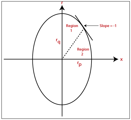
The equation of ellipse = p2 / rp2 + q2 / rq2 = 1
We will simplify the equation as follows-
p2 rq2 + q2 rp2 = rp2 rq2
We can represent the ellipse by following equation-
f (p, q) = rq2 p2 + rp2 q2 – rp2 rq2 …………………………. (1)
Now, there are three following conditions-
If
f (p, q) < 0
then
(p, q) is inside the ellipse boundary.
If
f (p, q) = 0
then
(p, q) is on the ellipse boundary.
If
f (p, q) > 0
then
(p, q) is outside the ellipse boundary.
Now,we partially differentiate the equation (1), and we get-
dp /dq = -2rq2p / 2rp2q
2rq2p >= 2rp2q {when we switch from region 1 to region 2}
Now, we will calculate the decision parameter (dk1) for region 1-
dk1 = (pk+1, qk – 1/2)
Now, we put the value in equation (1)
f (p, q) = rq2 (pk+1)2 + rp2 (qk – 1/2)2 – rp2 rq2 ………………………… (2)
Now, we calculate the next decision parameter (dk1+1)
dk1+1 = (pk+1+1, qk+1 – 1/2)
Now, we put the value of dk1+1 in equation (2)
dk1+1 = rq2 ((pk+1) +1)2 + rp2 (qk+1 – 1/2)2 – rp2 rq2
We simplify the equation (2) by {(A+B)2} and {(A-B)2 }
dk1+1 = rq2 [(pk+1)2 +12+2 (pk+1)]2 + rp2 [(qk+1)2 +1/4 –2(1/2) qk+1] – rp2 rq2
Now, we find the difference between dk1+1 and dk1
dk1+1 - dk1= rq2 [(pk+1)2+12+2(pk+1)]2+rp2 [(qk+1)2+1/4–qk+1]–rp2rq2 – rq2((pk+1) +1)2 + rp2 (qk+1 – 1/2)2 – rp2 rq2
dk1+1 = dk1+rq2 + 2 rq2(pk+1) +rp2 [(qk-1/2)- (qk-1/2)2] ……………. (3)
If
Decision parameter (dk1) < 0
Then
dk1+1 = dk1 + rq2 + 2 rq2 (pk+1)
If
Decision parameter (dk1) > 0
Then
dk1+1 = dk1 + rq2 + 2 rq2 (pk+1) – 2 rp2 qk+1
Now, we calculate the initial decision parameter dk1(0)
dk1(0) = rq2 + ¼ rp2 – rp2rq {For region 1}
Thus, we calculate the decision parameter (dk2) for region 2-
dk2 = (pk+1/2, qk – 1)
Now, we put the value of dk2 in equation (1)
dk2 = rq2 (pk +1/2)2 + rp2 (qk -1)2 – rp2 rq2
Now, we calculate the next decision parameter (dk2+1)
(dk2+1) = (pk+1 +1/2, qk+1 – 1)
Now, we put the value of dk2+2 in previous equation
dk2+1 = rq2 ((pk+1) +1/2)2 + rp2 (qk-1) – 1)2 – rp2 rq2
We simplify the equation and calculate the difference between dk2+1 and dk2. We get-
dk2+1 = dk2-2rp2 (qk -1) +rp2 +rq2 2 [(pk+1+1/2)2- (pk+1/2)2] ……………… (4)
Now, we check two conditions-
If
Decision parameter (dk2) < 0
Then
dk2+1 = dk2 -2 rp2qk+1 + rp2
If
Decision parameter (dk2) > 0
Then
dk2+1 = dk2 +2rq2 pk+1 -2 rp2 qk+1 +rp2
Now, we calculate the initial decision parameter dk2(0)
dk1(0) = rq2(pk +1/2)2 + rp2(qk -1) – rp2rq {For region 2}
Algorithm of Midpoint Ellipse Drawing
Step 1: First, we read rp and rq.
Step 2: Now we initialize starting coordinates as follow-
p = 0 and q =rq
Step 3: Wecalculate the initial value and decision parameter for region 1 as follow-
dk1 = r2q - r2p r2q + ¼ r2p
Step 4: Now, we initialize dp and dq as follows-
dp = 2r2qp
dq = 2r2pq
Step: 5 Now, we apply Do-while loop
Do
{plot (p, q)
If (dk1 < 0)
(p= p+1 and q = q)
dp = dp + 2r2q
dk1 = dk1 – dp + r2q
[dk1 = dk1 + 2r2qp +2r2q + r2q]
}
Else
(p= p+1 and q = q -1)
dp = dp + 2r2q
dq = dq - 2r2p
dk1 = dk1 + dp - dp + r2q
[dk1 = dk1 + 2r2qp +2r2q – (2r2pq - 2r2p) + r2q]
} while (dp < dq)
Step 6: Now,wecalculate the initial value and decision parameter for region 2 as follow-
dk2 = r2q (p + 1/2)2 + r2p (q-1)2 – r2p r2q
Step 7: Now, we again apply Do-while loop
Do
{plot (p, q)
If (dk2 < 0)
(p= p and q = q - 1)
dq = dp - 2r2p
dk2 = dk2 – dq + r2p
[dk2 = dk2 – (2r2pq - 2r2p) + r2p]
}
Else
(p= p+1 and q = q -1)
dq = dq - 2r2p
dp = dp + 2r2q
dk2 = dk2 + dp – dq + r2p
[dk2 = dk2 + 2r2qp +2r2q – (2r2pq - 2r2p) + r2q]
} while (q < 0)
Step 8: Thus, we calculate all the points of other quadrants.
Step 9: Stop.


Comments
Post a Comment